$$$$

12  First Examples

Highlights of this Chapter: We define infinite series and infinite products, and look at some examples where one can compute the sum exactly: telescoping and geometric series. We study the sums of reciprocal powers of $n$, and show that the harmonic series $\sum \frac{1}{n}$ diverges, whereas $\sum \frac{1}{n^2}$ converges.

We’ve met several types of sequences so far where its possible to precisely describe their terms, which basically fall into one of two categories: those with closed forms like $a_n=\frac{\sqrt{1+3n^2}}{2n+1}$ where each term is given explicitly in terms of $n$, and recursive sequences where each term is given in terms of the previous ones. The simples recursive sequences are defined by just iterating a single function, which we’ve successfully attacked with monotone convergence and the Contraction Mapping Theorem. Perhaps the next simplest recursive sequences are from iterating a process like addition or multiplication, so we will study these now.

Definition 12.1 (Series) A series $s_n$ is a recursive sequence defined in terms of another sequence $a_n$ by the recurrence relation $s_{n+1}=s_n+a_n$. Thus, the first terms of a series are $$s_0=a_0,s_1+a_0+a_1{s}_2=a_0+a_1+a_2\dots$$ We use summation notation to denote the terms of a series: $$s_n{=}_0+a_1+\cdots +a_n=\sum _{k=0}^n{a}_k$$

Remark 12.1. It is important to carefully distinguish between the sequence $a_n$ of terms being added up, and the sequence $s_n$ of partial sums.

When a series converges, we often denote its limit using summation notation as well. The traditional ‘calculus notation’ sets $n$ to infinity as the upper index; and another common notation is to list just the subset of integers over which we sum in as the lower bound: all of the following are acceptable

$$lim{s}_n=lim\sum _{k=0}^n{a}_k=\sum _{k=0}^{\mathrm{\infty }}{a}_k=\sum _{k\ge 0}{a}_k$$

Remark 12.2. Because the sum of any finitely many terms of a series is a finite number, we can remove any finite collection without changing whether or not the series converges. In particular, when proving convergence we are free to ignore the first finitely many terms when convenient. Because of this, we often will just write $\sum a_n$ when discussing a series, without giving any lower summation bound.

There are many important infinite series in mathematics: one that we encountered earlier is the Basel series first summed by Euler. $$\sum _{n\ge 1}\frac{1}{n^2}=\frac{{\pi }^2}{6}$$

When the sequences $a_n$ consists of functions of $x$, we may define an infinite series function for each $x$ at which it converges. These describe some of the most important functions in mathematics, such as the Riemann zeta function $$\zeta (s)=\sum _{n\ge 1}\frac{1}{n^s}$$

One of our big accomplishments to come in this class is to prove that exponential functions can be computed via infinite series, and in particular, the standard exponential of base $e$ has a very simple expression

$$\exp (x)=\sum _{n\ge 0}\frac{x^n}{n!}$$

The other infinite algebraic expression we can conjure up is infinite products:

Definition 12.2 (Infinite Products) An infinite product $p_n$ is a recursive sequence defined in terms of another sequence $a_n$ by the recurrence relation $p_{n+1}=p_n{a}_n$. Thus, the first terms of a series are $$s_0=a_0,s_1+a_0{a}_1{s}_2=a_0{a}_1{a}_2\dots$$ We use product notation to denote the terms of a series:_ $$s_n{=}_0{a}_1\cdots a_n=\prod _{k=0}^n{a}_k$$

Again, like for series, when such a sequence converges there are multiple common ways to write its limit:

$$lim{p}_n=lim\prod _{k=0}^n{p}_k=\prod _{k=0}^{\mathrm{\infty }}{p}_k=\prod _{k\ge 0}{p}_k$$

The first infinite product to occur in the mathematics literature is Viete’s Product for $\pi$

$$\frac{2}{\pi }=\frac{\sqrt{2}}{2}\frac{\sqrt{2+\sqrt{2}}}{2}\cdots$$

This product is derived from Archimedes’ side-doubling procedure for the areas of circumscribed $n$-gons; hence the collections of nested roots!

Another early and famous example being Wallis’ infinite product for $2/\pi$, which instead is derived from Euler’s infinite product for the sine function.

$$\frac{\pi }{2}=\prod _{n\ge 1}\frac{4n^2}{4n^2-1}$$ $$=\frac{2}{1}\frac{2}{3}\frac{4}{3}\frac{4}{5}\frac{6}{5}\frac{6}{7}\frac{8}{7}\frac{8}{9}\frac{10}{9}\frac{10}{11}\frac{12}{11}\frac{12}{13}\frac{14}{13}\frac{14}{15}\cdots$$

In 1976, the computer scientist N. Pippenger discovered a modification of Wallis’ product which converges to $e$:

$$\frac{e}{2}={\left(\frac{2}{1}\right)}^{\frac{1}{2}}{\left(\frac{2}{3}\frac{4}{3}\right)}^{\frac{1}{4}}{\left(\frac{4}{5}\frac{6}{5}\frac{6}{7}\frac{8}{7}\right)}^{\frac{1}{8}}{\left(\frac{8}{9}\frac{10}{9}\frac{10}{11}\frac{12}{11}\frac{12}{13}\frac{14}{13}\frac{14}{15}\frac{16}{15}\right)}^{\frac{1}{16}}\cdots$$

Pippenger wrote up his result as a paper…but due to the relatively ancient tradition of mathematics he was adding to - he decided to write it in Latin! The paper appears as “Formula nova pro numero cujus logarithmus hyperbolicus unitas est”. in IBM Research Report RC 6217. I am still trying to track down a copy of this! So if any of you are better at the internet than me, I would be very grateful if you could locate it.

Alluded to above, one of the most famous functions described by an infinite product is the sine function, which Euler expanded in his proof of the Basel sum $$\frac{\sin \pi x}{\pi x}=\prod _{n\ge 1}(1-\frac{x^2}{n^2})$$

AAs well as our friend the Riemann zeta function from above, which can be written as a product over all the primes! (Alluding to its deep connection to number theory)

$$\zeta (s)=\prod _{p\mathrm{prime}}\frac{1}{1-p^{-s}}$$

Perhaps in a calculus class you remember seeing many formulas for the convergence of series (we will prove them here in short order), but did not see many infinite products. The reason for this is that it is enough to study one class of these recursive sequences, once we really understand exponential functions and logarithms: we can use these to convert between the two. Because of this we too will focus most of our theoretical attention on series, though interesting products of historical significance will make several appearances.

12.0.1 Elementary Properties

To finish this introduction, we give several properties of infinite series which follow directly from their definition as limits of sequences of partial sums.

Definition 12.3 (Cauchy Criterion) A series $s_n=\sum a_n$ satisfies the Cauchy criterion if for every $\epsilon >0$ there is an $N$ such that for any $n,m>N$ we have $$\left|\sum _m^n{a}_k\right|<\epsilon$$

Exercise 12.1 Prove a series satisfies the Cauchy criterion if and only if its sequence of partial sums is a Cauchy sequence.

Proposition 12.1 (The Addition of Series) If $\sum a_n$ and $\sum b_n$ both converge, then the series $\sum (a_n+b_n)$ converges and $$\sum _{n\ge 0}(a_n+b_n)=\sum _{n\ge 0}{a}_n+\sum _{n\ge 0}{b}_n$$

Proof. For each $N$, let $A_N=\sum _{n=0}^N{a}_n$ and $B_N=\sum _{n=0}^N{b}_n$. Then the value of the infinite sums are $\sum _{n\ge 0}{a}_n=lim{A}_N$ and $\sum _{n\ge 0}{b}_n=lim{B}_N$. For any finite $N$, we can use the commutativity and associativity of addition to see $$\begin{array}{rl}\sum _{n=0}^N(a_n+b_n)& =(a_0+b_0)+(a_1+b_1)+\cdots +(a_N+b_N)\\ & =(a_0+a_1+\cdots +a_N)+(b_0+b_1+\cdots +b_N)\\ & =\sum _{n=0}^N{a}_n+\sum _{n=0}^N{b}_n\\ & =A_N+B_N\end{array}$$

Since $A_N$ and $B_N$ both converge by assumption, we can apply the limit law for sums to see $$lim(A_N+B_N)=lim{A}_N+lim{B}_N$$

Putting this all together we have proven what we want, $\sum _{n\ge 0}(a_n+b_n)$ exists, and equals the sum of $\sum _{n\ge 0}{a}_n$ and $\sum _{n\ge 0}{b}_n$.

Exercise 12.2 (Constant Multiple of a Series) Prove that if $\sum a_n$ is a convergent series and $k\in \mathbb{R}$ a constant, then the series $\sum k{a}_n$ is convergent, and $$\sum _{n\ge 0}k{a}_n=k\sum _{n\ge 0}{a}_n$$

Remark 12.3. Multiplying series is more subtle, as the terms of $\left(\sum _{n=0}^N{a}_n\right)\left(\sum _{n=0}^N{b}_n\right)$ are not just the pairwise products $a_n{b}_n$: we need to multiply it all out. The resulting construction is called the Cauchy Product, and we will later show that under the right conditions if $\sum a_n=A$ and $\sum b_n=B$ then the Cauchy product converges to $AB$.

Exercise 12.3 Let $\prod _{k\ge 1}{a}_k=\alpha$ and $\prod _{k\ge 1}{b}_k=\beta$ be convergent infinite products. Prove that $\prod _{k=1}{a}_k{b}_k$ converges, with limit $\alpha \beta$.

12.1 Telescoping Series

There are rare cases when we can sum a series directly, but these will prove very useful as basic series much as our basic sequences underlied much of our earlier work. The simplest way to directly sum a series is to find an exact formula for its partial sums, and telescoping series are a particularly nice example, where algebra makes this almost trivial

Definition 12.4 (Telescoping Series) A telescoping series is a series $\sum a_n$ where the terms themselves can be written as differences of consecutive terms of another sequence, for example if $a_n=t_{n-1}-t_n. 

Telescoping series are the epitome of a math problem that looks difficult, but is secretly easy. Once you can express the terms as differences, everything but the first and last cancels out! For example:

$$\begin{array}{rl}{s}_n& =\sum _{k=1}^n{a}_k\\ & =\sum _{k=1}^n(t_k-t_{k-1})\\ & =(t_n-t_{n-1})+(t_{n-1}-t_{n-2})+\cdots +(t_2-t_1)+(t_1-t_0)\\ & =t_n+(t_{n-1}-t_{n-1})+\cdots +(t_2-t_2)+(t_1-t_1)-t_0\\ & =t_n-t_0\end{array}$$

Thus, evaluating the sum is just as easy as evaluating the limit of $t_n$:

$$lim{s}_n=lim(t_n-t_0)=(lim{t}_n)-t_0$$

Thus, once a series has been identified as telescoping, often proving its convergence is straightforward: you get a direct formula for the partial sums, and then all that remains is to calculate the limit of a sequence. Because there are many ways a sequence might telescope its easier to look at examples than focus on the general theory.

Example 12.1 The sum $\sum _{k\ge 1}\frac{1}{k}-\frac{1}{k+1}$ telescopes. Writing out a partial sum $s_n$, everything collapses so $s_n=1-\frac{1}{n+1}$.

$$\begin{array}{rl}{s}_n& =(\frac{1}{n}-\frac{1}{n+1})+(\frac{1}{n-1}-\frac{1}{n})+\cdots +(\frac{1}{2}-\frac{1}{3})+(\frac{1}{1}-\frac{1}{2})\\ & =-\frac{1}{n+1}+(\frac{1}{n}-\frac{1}{n})+\cdots +(\frac{1}{2}-\frac{1}{2})+\frac{1}{1}\\ & =1-\frac{1}{n+1}\end{array}$$

Now we no longer have a series to deal with, as we’ve found the partial sums! All that remains is the sequence $s_n=1-\frac{1}{n+1}$. And this limit can be computed immediately from the limit laws:

$$s=lim{s}_n=1-lim\frac{1}{n+1}=1$$

Of course, sometimes a bit of algebra needs to be done to reveal that a series is telescoping:

Example 12.2 Compute the sum of the series $$\sum _{n\ge 1}\frac{1}{n(n+1)}$$

Performing a partial fractions decomposition to $\frac{1}{n(n+1)}$ we seek $A,B$ with $\frac{A}{n}+\frac{B}{n+1}=\frac{1}{n(n+1)}$ which is satisfied by $A=1,B=-1$, so $$\frac{1}{n(n+1)}=\frac{1}{n}-\frac{1}{n+1}$$ Thus our series telescopes, with partial sums $$\sum _{n=1}^N\frac{1}{n(n+1)}=(1-\frac{1}{2})+(\frac{1}{2}-\frac{1}{3})+\cdots +(\frac{1}{N-1}-\frac{1}{N})=1-\frac{1}{N}$$

Taking the limit

$$\sum _{n\ge 1}\frac{1}{n(n+1)}=\underset{N}{lim}\sum _{n=1}^N\frac{1}{n(n+1)}=lim1-\frac{1}{N}=1$$

Telescoping series don’t need to cancel consecutive terms, but rather it can take a bit of time before the telescoping begins:

Example 12.3 Compute the sum of the series

$$\sum _{k\ge 1}\frac{1}{k^2+3k}$$

Doing partial fractions to the term $1/(k^2+3k)$ we find $$\frac{1}{k^2+3k}=\frac{2}{k(k+3)}=\frac{1}{3}(\frac{1}{k}-\frac{1}{k+3})$$

We’ll ignore the factor of $1/3$ while doing some scratch work below but be careful to bring it back later. Adding up the first two terms we don’t see any cancellations like we expect of a telescoping series

$$(1-\frac{1}{3})+(\frac{1}{2}-\frac{1}{4})$$

But, after more terms the cancellations begin: the sixth term is

$$(1-\frac{1}{3})+(\frac{1}{2}-\frac{1}{4})+(\frac{1}{3}-\frac{1}{5})+(\frac{1}{4}-\frac{1}{6})+(\frac{1}{5}-\frac{1}{7})+(\frac{1}{6}-\frac{1}{8})$$ $$=1+\frac{1}{2}-\frac{1}{7}-\frac{1}{8}$$

Seeing the pattern here, you can prove by induction that the $N^{th}$ term is $$\frac{1}{3}(1+\frac{1}{2}-\frac{1}{N+1}-\frac{1}{N+2})$$

So, taking the limit as the number of terms we add goes to infinity we can use the limit laws together with $1/N\to 0$ to conclude $$\sum _{k\ge 1}\frac{1}{k^2+3k}=lim\frac{1}{3}(1+\frac{1}{2}-\frac{1}{N+1}-\frac{1}{N+2})$$ $$=\frac{1}{3}(1+\frac{1}{2}-0-0)=\frac{1}{3}\frac{3}{2}=\frac{1}{2}$$

Exercise 12.4 Show that the following series is telescoping, and then find its sum $$\sum _{n\ge 1}\frac{1}{4n^2-1}$$ Hint: factor the denominator, and do a partial fractions decomposition!

A telescoping product is defined analogously

Definition 12.5 (Telescoping Product) A telescoping product is a product $\prod a_n$ where the terms themselves can be written as ratios of consecutive terms of another sequence, for example $a_n=\frac{t_n}{t_{n-1}}$.

Exercise 12.5 Find the value of the following infinte product by showing its telescoping and computing an exact formula for its partial sums: $$\prod _{n\ge 5}\left(\frac{1}{n^2}\right)$$

An example of historical importance is below:

Example 12.4 (Viete’s Product for $\pi$) Viete’s infinite product $\frac{2}{\pi }=\frac{\sqrt{2}}{2}\frac{\sqrt{2+\sqrt{2}}}{2}\cdots$ which we derived back in the introductory historical chapter to this text from an infinite application of the half angle formula, can also be derived as a telescoping product, where each term represents the ratio of the area of a circumscribed polygon and and its side-doubled cousin.

• The first term, $\sqrt{2}/2$ is the ratio of the area of an square to a octagon.
• The second term, $\sqrt{2+\sqrt{2}}/2$ is the ratio of the area of a octagon to an 16-gon.
• The $n^{th}$ term is the ratio of the area of a $2^{n+1}$-gon to a $2^{n+2}$-gon.

When multiplying these all together, the intermediaries cancel, and in the limit this gives the ratio of the area of a square to the area of a circle.

12.2 Geometric Series

Definition 12.6 A series $\sum a_n$ is geometric if all consecutive terms share a common ratio: that is, there is some $r\in \mathbb{R}$ with $a_n/a_{n-1}=r$ for all $n$.

In this case we can see inductively that the terms of the series are all of the form $a{r}^n$. Thus, often we factor out the $a$ and consider just series like $\sum r^n$.

Exercise 12.6 (Geometric Partial Sums) For any real $r$, the partial sum of the geometric series is: $$1+r+r^2+\cdots +r^n=\sum _{k=0}^n{r}^n=\frac{1-r^{n+1}}{1-r}$$

Like telescoping series, now that we have explicitly computed the partial sums, we can find the exact value by just taking a limit.

Theorem 12.1 If $|r|<1$ then $\sum r^n$ converges, and $$\sum _{k=0}^{\mathrm{\infty }}{r}^k=\frac{1}{1-r}$$

Conversely if $|r|>1$, the geometric series $\sum r^n$ diverges.

Proof. We begin with the case $|r|<1$. By the partial sum formula, we have
$$\sum _{n\ge 0}{r}^n=lim\sum _{k=0}^n{r}^n=lim\frac{1-r^{n+1}}{1-r}$$ Since $|r|<1$, we know that $r^n\to 0$, and so $r^{n+1}=r{r}^n\to 0$ by the limit theorems (or by truncating the first term of the sequence). Again by the limit theorems, we may then calculate $$lim\frac{1-r^{n+1}1-r}{=}\frac{1-lim{r}^{n+1}}{1-r}=\frac{1-0}{1-r}=\frac{1}{1-r}$$

For $|r|>1$, we directly see the sum is unbounded as each $r^k>1^k=1$ so $$s_N=\sum _{k=0}^N{r}^k>1+1+\cdots +1=N+1$$ As convergent sequences are bounded, this must diverge.

Exercise 12.7 Show if $r<-1$ that $\sum r^k$ diverges.

Hint: look at the subsequence $s_0,s_2,s_4,s_6\dots$ of partial sums.

Remark 12.4. Its often useful to commit to memory the formula also for when the sum starts at $1$: $$\sum _{k\ge 1}{r}^k=\frac{r}{1-r}$$

Example 12.5 What should the infinite decimal $0.99999\cdots$ mean?

Because this holds for all values of $r$ between $-1$ and $1$, this gives us our first taste of a function defined as an infinite series. For any $x\in (-1,1)$ we may define the function $$f(x)=1+x+x^2+x^3+\cdots +x^n+\cdots$$ and the argument above shows that $f(x)=1/(1-x)$. Thus, we have two expressions of the same function: one in terms of an infinite sum, and one in terms of familiar algebraic operations. This sort of thing will prove extremely useful in the future, where switching between these two viewpoints can often help us overcome difficult problems. $$\frac{1}{1-x}=1+x+x^2+x^3+x^4+x^5+\cdots$$

The theory of geometric series began with Archimedes’ famous paper The Quadrature of the Parabola, and we can now make his final argument rigorous in a modern form. (We will not make rigorous the first steps of the argument, which deal mainly in geometry, but re review them briefly here)

Archimedes’ big idea was to divide a parabolic up into triangles recursively by drawing the largest triangle which inscribes in the segment. This divides the parabolic segment into a triangle and two smaller parabolic segments, on which the process repeats.

Archimedes’ infinite construction of the parabolic segment from triangles

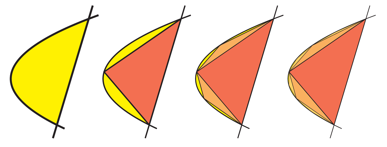
Denote by $T_n$ the sum of the areas of the triangles which appear at the $n$^{th}$ stage of this process (so $T_0$ is one triangle $T_1$ consists of two triangles, $T_2$ of four triangles, etc). Through clever use of the geometry of parabolas, archimedes shows that $T_{n+1}=\frac{1}{4}{T}_n$. And through further clever geometry, Archimedes argues that in the limit as $n\to \mathrm{\infty }$, these triangles completely fill the parabola, so its area is the sum of their areas. That is

$$\mathrm{Area}=\sum _{n\ge 0}{T}_n=\sum _{n\ge 0}\frac{T_0}{4^n}=T_0\sum _{n\ge 0}{\left(\frac{1}{4}\right)}^n$$

Summing this geometric series yields the celebrated result:

Theorem 12.2 The area of the segment bounded by a parabola and a chord is $4/3^{rd}$s the area of the largest inscribed triangle.

12.3 Summing Reciprocals

Some of the most natural infinite series to consider are the sums of reciprocal natural numbers and their powers. The simplest of these is simply

$$\sum _{n\ge 1}\frac{1}{n}=1+\frac{1}{2}+\frac{1}{3}+\frac{1}{4}+\cdots +\frac{1}{n}+\cdots$$

and called the Harmonic Series (named after a distant connection to music). Other common examples are $\sum \frac{1}{n^2}$ or $\sum 1n^3$, etc. These arise everywhere throughout analysis, and find important applications in physics, number theory and beyond. In this final section of our introductory chapter we use what we’ve learned to calculate their values:

Theorem 12.3 (Divergence of the Harmonic Series) The harmonic series $\sum _{n\ge 1}\frac{1}{n}$ diverges.

Proof. Let $s_N=\sum _{n=1}^N\frac{1}{N}$ denote the partial sums of the harmonic series, and note we have the following inequality relating $s_{2N}$ with $s_N$:

$$\begin{array}{rl}{s}_{2N}& =1+\frac{1}{2}+\frac{1}{3}+\frac{1}{4}+\frac{1}{5}+\frac{1}{6}+\cdots +\frac{1}{2N-1}+\frac{1}{2N}\\ & =1+\frac{1}{2}+(\frac{1}{3}+\frac{1}{4})+(\frac{1}{5}+\frac{1}{6})+\cdots +(\frac{1}{2N-1}+\frac{1}{2N})\\ & >1+\frac{1}{2}+(\frac{1}{4}+\frac{1}{4})+(\frac{1}{6}+\frac{1}{6})+\cdots +(\frac{1}{2N}+\frac{1}{2N})\\ & =1+\frac{1}{2}+\frac{1}{2}+\frac{1}{3}+\cdots +\frac{1}{N}\\ & =\frac{1}{2}+(1+\frac{1}{2}+\frac{1}{3}+\cdots +\frac{1}{N})\\ & =\frac{1}{2}+s_N\end{array}$$

Now assume for the sake of contradiction that the harmonic series does converge, so $lim{s}_N=L$ exists. Then all subsequences converge to the same limit, so restricting to the even subsequence, $lim{s}_{2N}=L$ as well. But the inequality above ensures $s_{2N}>\frac{1}{2}+s_N$, and applying the limit theorems yields $$lim{s}_{2N}>\frac{1}{2}=lim{s}_N⟹L>\frac{1}{2}+L$$

Subtracting $L$ from both sides and multiplying by $2$ gives $0>1$, a contradiction.

Exercise 12.8 Give an alternate proof that the harmonic series $\sum \frac{1}{n}$ diverges, by comparing it with the partial sums of $$1,1/2,1/4,1/4,1/8,1/8,1/8,1/8,1/16,...$$

Hint: show that for each $N$ the partial sum of the harmonic series is greater than the partial sums of this series. But then show the partial sums of this series are unbounded: for any integer $k$ we can find a point where the sum surpasses $k$. This means the partial sums of the harmonic series are unbounded: but we know all convergent series are bounded! Thus the harmonic series cannot be convergent.

Theorem 12.4 (Convergence of the Reciprocal Squares) The series $\sum _{n\ge 1}\frac{1}{n^2}$ converges.

Proof. Let $s_N$ denote the partial sums of the series. Since $1/n^2>0$ for all $n$, we see the sequence $s_N$ is monotone increasing for all $N$, $$s_N=s_{N-1}+\frac{1}{N^2}>s_{N-1}$$

Thus to prove it converges we need only show its bounded above (and then apply the Monotone Convergence Theorem). As a first step, note that for every $n>1$, we know $n-1<n$ and so $\frac{1}{n^2}<\frac{1}{n(n-1)}$. Adding these up, we see $$\sum _{n=2}^N\frac{1}{n^2}<\sum _{n=2}^N\frac{1}{n(n-1)}$$ This latter sum telescopes, so we can compute its partial sums directly: $$\sum _{n=2}^N\frac{1}{n(n-1)}=\sum _{n=2}^N(\frac{1}{n-1}-\frac{1}{n})=(1-\frac{1}{2})+(\frac{1}{2}-\frac{1}{3})+\cdots +(\frac{1}{N-1}-\frac{1}{N})=1-\frac{1}{N}$$

Thus, for all $N$ we see $\sum _{n=2}^N\frac{1}{n^2}<1-\frac{1}{N^2}<1$, so $$\sum _{n=1}^N\frac{1}{n^2}=1+\sum _{n=2}^N\frac{1}{n^2}<1+1=2$$

Together, our sequence of partial sums is monotone increasing and bounded above by 2, so its convergent.

While proving $\sum \frac{1}{n^2}$ is convergent was relatively straightforward, finding its value is what brought Lehonard Euler his first mathematical fame, when proved it equals exactly ${\pi }^2/6$.

Exercise 12.9 Prove that for $s\ge 2$ that $\sum \frac{1}{n^s}$ converges.

Hint: show its monotone; and shows its bounded by comparing partial sums with those of $\sum \frac{1}{n^2}$. which we know converges.

12.4 Problems

12.4.1 The Koch Fractal

The Koch Snowflake is a fractal, defined as the limit of an infinite process starting from a single equilateral triangle. To go from one level to the next, every line segment of the previous level is divided into thirds, and the middle third replaced with the other two sides of an equilateral triangle built on that side.

The Koch subdivision rule: replace the middle third of every line segment with the other two sides of an equilateral triangle.

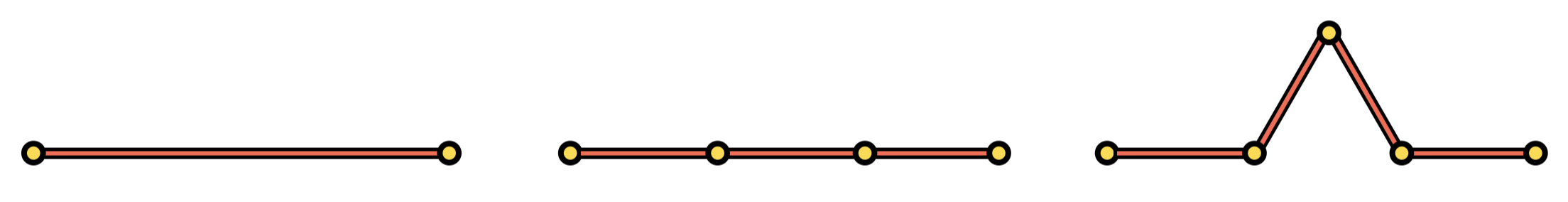
Doing this to every line segment quickly turns the triangle into a spiky snowflake like shape, hence the name. Denote by $K_n$ the result of the $n^{th}$ level of this procedure.

The first six stages $K_0,K_1,K_2,K_3,K_4$ and $K_5$ of the Koch snowflake procedure. $K_{\mathrm{\infty }}$ is the fractal itself.

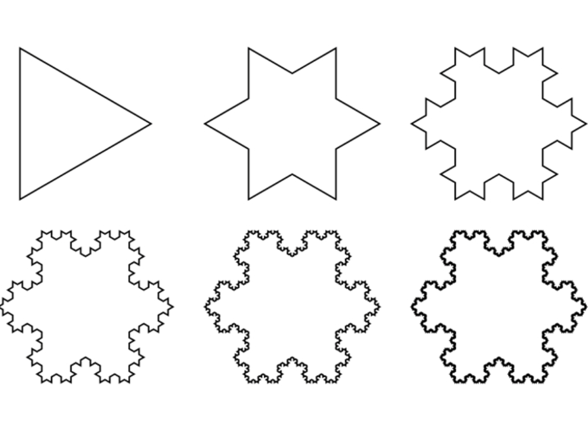
Say the initial triangle at level $0$ has perimeter $P$, and area $A$. Then we can define the numbers $P_n$ to be the perimeter of the $n^{th}$ level, and $A_n$ to be the area of the $n^{th}$ level..

Exercise 12.10 (The Koch Snowflake Length) What are the perimeters $P_1,P_2$ and $P_3$ of the first iterations? From this conjecture (and then prove by induction) a formula for the perimeter $P_n$ and prove that $P_n$ diverges. Thus, the limit cannot be assigned a length!

Next we turn to the area: recall that the area of an equilateral triangle can be given in terms of its side length as $A=\frac{\sqrt{3}}{2}{s}^2$

Exercise 12.11 (The Koch Snowflake Area) What are the areas $A_1,A_2$ and $A_3$ in terms of the original area $A$? Find an infinite series that represents the area of the $n^{th}$ stage $A_n$, and prove that your formula is correct by induction.

Now, use what we know about geometric series to prove that this converges: in the limit, the Koch snowflake has a finite area even though its perimeter diverges!